Optimization

Optimization

Professor:

Paul Wollan

Office Hours:

Class Times:

Announcements

Note that the class originally scheduled for Thursday morning has been moved to Wednesday 8:30 - 10 in Aula G50.
There will be no class the week of 18 - 22 March.
The results for the June 17 exam can be found here.
The results for the July 21 exam can be found here. Please confirm if you would like to finalize the grade by email.
The results for the September 19 exam can be found here. Please confirm if you would like to finalize the grade by email.

Prerequisites:

The course requires a minimal acquaintance with discrete mathematics including mathematical induction and the basic notions of graph theory. All other necessary background will be covered in the course itself. Description:

A central problem of combinatorial optimization seeks to minimize (or maximize) a linear function on a set of variables subject to a set of linear constraints. The generality of this problem yields a huge number of applications both in theoretical computer science as well in the search for solutions to real world problems. We examine how to solve such problems both from a theoretical as well as practical point of view. The general topics covered in the course are:

Network flow

Linear Programming

Integer Programming

Recommended texts:

Combinatorial Optimization, William Cook, William Cunningham, William Pulleybank, and Lex Schrijver, Wiley 1998
Understanding and Using Linear Programming, Jiri Matousek and Bernd Gartner, Springer 2007
Introduction to Linear Optimization, Dimitris Bertsimas and John Tsitsiklis, Athena Scientific 1997.

Class summaries

Class 1:

Definitions: Graph, vertices, edges, flow in a graph, flow problem, residual graph, augmenting a flow.

Ford-Fulkerson algorithm for finding a flow. Combinatorial Optimization, pages 40 - 43

Definitions: Cut in a graph, capacity of a cut.

Class 2:

Theorem: maximum flow in a graph is equal to the minimum capacity of a cut. Combinatorial Optimization, Theorem 3.5

Edmonds-Karp algorithm for finding a flow. Proof that the Edmonds-Karp algorithm terminates in O(nm) augmentations of the flow. Combinatorial Optimization, pages 44 - 45

Class 3:

Completion of the proof of correctness of the Edmonds-Karp algorithm for finding a flow. Combinatorial Optimization, pages 44 - 45

Application of Max-flow/Min-cut: Menger's Theorem for edge disjoint paths.

Class 4:

Definitions: Linear program, objective function, constraints, feasible solution, optimal solution, Understanding and Using Linear Programming, Chapter 1.

Proposition: If a linear program has two distinct optimal solutions, then it has infinitely many optimal solutions.

Examples of Linear Programming: resource allocation, network flow. Understanding and Using Linear Programming, pages 11 - 15.

Class 5:

Example of Linear Programming: Largest disk in a convex polygon. Understanding and Using Linear Programming, pages 23 - 26.

Definitions: equation form of a linear program, slack variables, Basic feasible solution, basic variables, non-basic variables, feasible basis Understanding and Using Linear Programming, Chapter 4.

Proposition: A feasible solution x of a linear program in equational form is basic if and only if the columns of the matrix A_K are linearly independent where K = { i : 1 ≤ i ≤ n, x _i > 0}. Understanding and Using Linear Programming, Lemma 4.2.1.

Proposition: A feasible basis B defines a unique solution x to Ax = b, x ≥ 0. Understanding and Using Linear Programming, Proposition 4.2.2.

Class 6:

Theorem: Consider a linear program in equational form: max c^T x subject to Ax = b, x ≥ 0.

If there exists at least one feasible solution and the objective function is bounded from above on the set of feasible solutions, then there exists an optimal solution.
If an optimal solution exists, then there exists a basic feasible solution which is optimal.

Understanding and Using Linear Programming

Class 7:

Definitions: Convex set, convex hull, convex combination, hyperplane, closed half-space, polyhedron, polytope, dimension of a polyhedron, vertex of a polyhedron, edge of a polyhedron Understanding and Using Linear Programming, Chapter 4.

Proposition: Let x₁,...,x_n in Rⁿ. Let C be the convex hull of x₁,...,x_n and let C' be the set of convex combinations of x₁,...,x_n. Then C' = C. Understanding and Using Linear Programming, Proposition 4.3.1.

Theorem: Let P be the set of feasible solutions of a linear program in equational form. Then for all v ∈ P, v is a vertex of P if and only if v is a basic feasible solution to the linear program. Understanding and Using Linear Programming, Theorem 4.4.1.

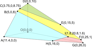
Solution to the problem presented in class.

Class 8:

Example of the simplex method. Understanding and Using Linear Programming, pages 57 - 60.

Definitions: tableau, pivot. Understanding and Using Linear Programming, Chapter 5.

Proposition: For every feasible basis B of a linear program in equational form, the tableau T(B) is uniquely determined by B. Understanding and Using Linear Programming, Proposition 5.5.1.

Class 9:

Discussion: Unboundedness, infeasibility, and degeneracy in linear programs. See Understanding and Using Linear Programming, pages 61 - 65.

Class 10:

Examples of pivot rules, including Bland's rule.

Proposition: Algebraic conditions for the tableau T(B) for a feasible basis B which guarantee a pivot will result in a feasible basis B' = (B - {u}) ∪ {v}. Understanding and Using Linear Programming, Proposition 5.6.1.

Class 11:

Definitions: fickle variables.

Proposition: Let B₁,...,B_k be feasible bases for a linear program in equational form such that T(B₁) - T(B₂) - ... - T(B_k) - T(B₁) cycle with respect to a fixed pivoting rule. Let F be the set of indices of fickle variables in the cycle. Then there exists a basic feasible solution x such that for all j, 1 ≤ j ≤ k, x is the basic feasible solution associated to B_j and for all i such that x_i ∈ F, x_i = 0.

Theorem: The simplex method with pivoting according to Bland's rule does not cycle. Understanding and Using Linear Programming, Theorem 5.8.1.

Class 12:

Theorem: The simplex method with pivoting according to Bland's rule does not cycle. Understanding and Using Linear Programming, Theorem 5.8.1. (completion of the proof)

Class 13:

Example of a linear program which cycles for a specific pivot rule. See here for the explicit example as well as a discussion of the construction of such examples.

Definitions: dual linear program, primal linear program.

Proposition (Weak duality theorem): Consider the linear program: max c^T x subject to Ax ≤ b, x ≥ 0 and its dual linear program min b^T y subject to A^Ty ≥ c, y ≥ 0. If x and y are feasible solutions to the primal and dual linear programs, respectively, then c^T x ≤ b^T y. Understanding and Using Linear Programming, Theorem 6.1.1.

Class 14:

Discussion of the dual for a general linear program. See Understanding and Using Linear Programming, pages 84 - 86.

Proposition: Let P be a linear program and D the dual of P. Then the dual of D is the linear program P.

Theorem (Strong duality theorem): Consider the linear program (P): max c^T x subject to Ax ≤ b, x ≥ 0 and its dual linear program (D) min b^T y subject to A^Ty ≥ c, y ≥ 0. Exactly one of the following holds:

neither (P) nor (D) is feasible;
(P) is feasible and un bounded while (D) is not feasible;
(D) is feasible and un bounded while (P) is not feasible;
both (P) and (D) are feasible and in this case both are bounded and have the same optimum.